Monitoring Query Performance
The initial step in query tuning involves a thorough analysis of the query plan and its execution. The query plan and execution details illuminate how SQreamDB handles a query and pinpoint where time resources are consumed. This document offers a comprehensive guide on analyzing query performance through execution plans, with a specific emphasis on recognizing bottlenecks and exploring potential optimization strategies to enhance query efficiency.
It’s important to note that performance tuning approaches can vary for each query, necessitating adaptation of recommendations and tips to suit specific workloads. Additionally, for further insights into data loading considerations and other best practices, refer to our Optimization and Best Practices guide.
Setting Up System Monitoring Preferences
By default, SQreamDB automatically logs execution details for any query that runs longer than 60 seconds. This means that by default, queries shorter than 60 seconds are not logged. You can adjust this parameter to your own preference.
Adjusting the Logging Frequency
To customize statement logging frequency to be more frequent, consider reducing the interval from the default 60 seconds to a shorter duration like 5 or 10 seconds. This adjustment can be made by modifying the nodeInfoLoggingSec in your SQreamDB configuration files and setting the parameter to your preferred value.
{
   "compileFlags":{
   },
   "runtimeFlags":{
   },
   "runtimeGlobalFlags":{
      "nodeInfoLoggingSec" : 5,
   },
   "server":{
   }
}
After customizing the frequency, please restart your SQreamDB cluster. Execution plan details are logged to the default SQreamDB log directory as message type 200.
You can access these log details by using a text viewer or by creating a dedicated foreign table to store the logs in a SQreamDB table.
Creating a Dedicated Foreign Table to Store Log Details
Utilizing a SQreamDB table for storing and accessing log details helps simplify log management by avoiding direct handling of raw logs.
To create a foreign table for storing your log details, use the following table DDL:
CREATE FOREIGN TABLE logs (
  start_marker TEXT,
  row_id BIGINT,
  timestamp DATETIME,
  message_level TEXT,
  thread_id TEXT,
  worker_hostname TEXT,
  worker_port INT,
  connection_id INT,
  database_name TEXT,
  user_name TEXT,
  statement_id INT,
  service_name TEXT,
  message_type_id INT,
  message TEXT,
  end_message TEXT
)
WRAPPER
  csv_fdw
OPTIONS
  (
    LOCATION = '/home/rhendricks/sqream_storage/logs/**/sqream*.log',
    DELIMITER = '|'
  );
Use the following query structure as an example to view previously logged execution plans:
SELECT
  message
FROM
  logs
WHERE
  message_type_id = 200
  AND timestamp BETWEEN '2020-06-11' AND '2020-06-13';

message
---------------------------------------------------------------------------------------------------------------------------------
SELECT *,coalesce((depdelay > 15),false) AS isdepdelayed FROM ontime WHERE year IN (2005, 2006, 2007, 2008, 2009, 2010)

1,PushToNetworkQueue  ,10354468,10,1035446,2020-06-12 20:41:42,-1,,,,13.55
2,Rechunk             ,10354468,10,1035446,2020-06-12 20:41:42,1,,,,0.10
3,ReorderInput        ,10354468,10,1035446,2020-06-12 20:41:42,2,,,,0.00
4,DeferredGather      ,10354468,10,1035446,2020-06-12 20:41:42,3,,,,1.23
5,ReorderInput        ,10354468,10,1035446,2020-06-12 20:41:41,4,,,,0.01
6,GpuToCpu            ,10354468,10,1035446,2020-06-12 20:41:41,5,,,,0.07
7,GpuTransform        ,10354468,10,1035446,2020-06-12 20:41:41,6,,,,0.02
8,ReorderInput        ,10354468,10,1035446,2020-06-12 20:41:41,7,,,,0.00
9,Filter              ,10354468,10,1035446,2020-06-12 20:41:41,8,,,,0.07
10,GpuTransform        ,10485760,10,1048576,2020-06-12 20:41:41,9,,,,0.07
11,GpuDecompress       ,10485760,10,1048576,2020-06-12 20:41:41,10,,,,0.03
12,GpuTransform        ,10485760,10,1048576,2020-06-12 20:41:41,11,,,,0.22
13,CpuToGpu            ,10485760,10,1048576,2020-06-12 20:41:41,12,,,,0.76
14,ReorderInput        ,10485760,10,1048576,2020-06-12 20:41:40,13,,,,0.11
15,Rechunk             ,10485760,10,1048576,2020-06-12 20:41:40,14,,,,5.58
16,CpuDecompress       ,10485760,10,1048576,2020-06-12 20:41:34,15,,,,0.04
17,ReadTable           ,10485760,10,1048576,2020-06-12 20:41:34,16,832MB,,public.ontime,0.55
Using the SHOW_NODE_INFO Command
The SHOW_NODE_INFO command provides a snapshot of the current query plan. Similar to periodically-logged execution plans, SHOW_NODE_INFO displays the compiler’s execution plan and runtime statistics for a specified statement at the moment of execution.
You can execute the SHOW_NODE_INFO utility function using sqream sql, SQream Studio Editor, or other third party tool.
In this example, we inspect a statement with statement ID of 176:
SELECT
  SHOW_NODE_INFO(176);

stmt_id | node_id | node_type          | rows | chunks | avg_rows_in_chunk | time                | parent_node_id | read | write | comment    | timeSum
--------+---------+--------------------+------+--------+-------------------+---------------------+----------------+------+-------+------------+--------
    176 |       1 | PushToNetworkQueue |    1 |      1 |                 1 | 2019-12-25 23:53:13 |             -1 |      |       |            |  0.0025
    176 |       2 | Rechunk            |    1 |      1 |                 1 | 2019-12-25 23:53:13 |              1 |      |       |            |       0
    176 |       3 | GpuToCpu           |    1 |      1 |                 1 | 2019-12-25 23:53:13 |              2 |      |       |            |       0
    176 |       4 | ReorderInput       |    1 |      1 |                 1 | 2019-12-25 23:53:13 |              3 |      |       |            |       0
    176 |       5 | Filter             |    1 |      1 |                 1 | 2019-12-25 23:53:13 |              4 |      |       |            |  0.0002
    176 |       6 | GpuTransform       |  457 |      1 |               457 | 2019-12-25 23:53:13 |              5 |      |       |            |  0.0002
    176 |       7 | GpuDecompress      |  457 |      1 |               457 | 2019-12-25 23:53:13 |              6 |      |       |            |       0
    176 |       8 | CpuToGpu           |  457 |      1 |               457 | 2019-12-25 23:53:13 |              7 |      |       |            |  0.0003
    176 |       9 | Rechunk            |  457 |      1 |               457 | 2019-12-25 23:53:13 |              8 |      |       |            |       0
    176 |      10 | CpuDecompress      |  457 |      1 |               457 | 2019-12-25 23:53:13 |              9 |      |       |            |       0
    176 |      11 | ReadTable          |  457 |      1 |               457 | 2019-12-25 23:53:13 |             10 | 4MB  |       | public.nba |  0.0004
You may also download the query execution plan to a CSV file using the Execution Details View feature.
Understanding the Query Execution Plan Output
Both SHOW_NODE_INFO and the logged execution plans represents the query plan as a graph hierarchy, with data separated into different columns.
Each row represents a single logical database operation, which is also called a node or chunk producer. A node reports
several metrics during query execution, such as how much data it has read and written, how many chunks and rows, and how much time has elapsed.
Consider the example SHOW_NODE_INFO presented above. The source node with ID #11 (ReadTable), has a parent node ID #10
(CpuDecompress). If we were to draw this out in a graph, it’d look like this:
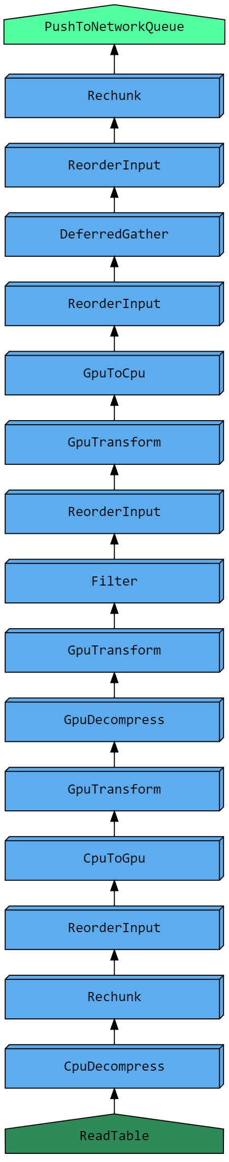
This graph explains how the query execution details are arranged in a logical order, from the bottom up.
The last node, also called the sink, has a parent node ID of -1, meaning it has no parent. This is typically a node that sends data over the network or into a table.
When using SHOW_NODE_INFO, a tabular representation of the currently running statement execution is presented. See the examples below to understand how the query execution plan is instrumental in identifying bottlenecks and optimizing long-running statements.
Information Presented in the Execution Plan
If the statement has finished, or the statment ID does not exist, the utility returns an empty result set.
Commonly Seen Nodes
Column name |
Execution location |
Description |
|---|---|---|
|
CPU |
Decompression operation, common for longer |
|
CPU |
A non-indexed nested loop join, performed on the CPU |
|
CPU |
A reduce process performed on the CPU, primarily with |
|
An operation that moves data to or from the GPU for processing |
|
|
CPU |
A transform operation performed on the CPU, usually a scalar function |
|
CPU |
Merges the results of GPU operations with a result set |
|
GPU |
Removes duplicate rows (usually as part of the |
|
CPU |
The merge operation of the |
|
GPU |
A filtering operation, such as a |
|
GPU |
Decompression operation |
|
GPU |
An operation to optimize part of the merger phases in the GPU |
|
GPU |
A transformation operation such as a type cast or scalar function |
|
CPU |
Validates external file paths for foreign data wrappers, expanding directories and GLOB patterns |
|
GPU |
A non-indexed nested loop join, performed on the GPU |
|
CPU |
A CSV parser, used after |
|
CPU |
Sends result sets to a client connected over the network |
|
CPU |
Reads external flat-files |
|
CPU |
Reads data from a standard table stored on disk |
|
Reorganize multiple small chunks into a full chunk. Commonly found after joins and when HIGH_SELECTIVITY is used |
|
|
GPU |
A reduction operation, such as a |
|
GPU |
A merge operation of a reduction operation, helps operate on larger-than-RAM data |
|
Change the order of arguments in preparation for the next operation |
|
|
GPU |
Gathers additional columns for the result |
|
GPU |
Sort operation |
|
Take the first N rows from each chunk, to optimize |
|
|
Limits the input size, when used with |
|
|
CPU |
Executes a user defined function |
|
Combines two sources of data when |
|
|
GPU |
Executes a non-ranking window function |
|
GPU |
Executes a ranking window function |
|
CPU |
Writes the result set to a standard table stored on disk |
Tip
The full list of nodes appears in the Node types table, as part of the SHOW_NODE_INFO reference.
Examples
Typically, examining the top three longest running nodes (detailed in the timeSum column) can highlight major bottlenecks. The following examples will demonstrate how to identify and address common issues.
Spooling to Disk
When SQreamDB doesn’t have enough RAM to process a statement, it will temporarily store overflow data in the temp folder on the storage disk. While this ensures that statements complete processing, it can significantly slow down performance. It’s important to identify these statements to assess cluster configuration and potentially optimize statement size.
To identify statements that spill data to disk, check the write column in the execution details. Nodes that write to disk will display a value (in megabytes) in this column. Common nodes that may write spillover data include Join and LoopJoin.
Identifying the Offending Nodes
Run a query.
This example is from the TPC-H benchmark:
SELECT
  o_year,
  SUM(
    CASE
      WHEN nation = 'BRAZIL' THEN volume
      ELSE 0
    END
  ) / SUM(volume) AS mkt_share
FROM
  (
    SELECT
      datepart(YEAR, o_orderdate) AS o_year,
      l_extendedprice * (1 - l_discount / 100.0) AS volume,
      n2.n_name AS nation
    FROM
      lineitem
      JOIN part ON p_partkey = CAST (l_partkey AS INT)
      JOIN orders ON l_orderkey = o_orderkey
      JOIN customer ON o_custkey = c_custkey
      JOIN nation n1 ON c_nationkey = n1.n_nationkey
      JOIN region ON n1.n_regionkey = r_regionkey
      JOIN supplier ON s_suppkey = l_suppkey
      JOIN nation n2 ON s_nationkey = n2.n_nationkey
    WHERE
      o_orderdate BETWEEN '1995-01-01' AND '1996-12-31'
  ) AS all_nations
GROUP BY
  o_year
ORDER BY
  o_year;
Use a foreign table or
SHOW_NODE_INFOto view the execution information.This statement is made up of 199 nodes, starting from a
ReadTable, and finishes by returning only 2 results to the client.The execution below has been shortened, but note the highlighted rows for
LoopJoin:SELECT message FROM logs WHERE message_type_id = 200 LIMIT 1; message ----------------------------------------------------------------------------------------- SELECT o_year, SUM(CASE WHEN nation = 'BRAZIL' THEN volume ELSE 0 END) / SUM(volume) AS mkt_share : FROM (SELECT datepart(YEAR,o_orderdate) AS o_year, : l_extendedprice*(1 - l_discount / 100.0) AS volume, : n2.n_name AS nation : FROM lineitem : JOIN part ON p_partkey = CAST (l_partkey AS INT) : JOIN orders ON l_orderkey = o_orderkey : JOIN customer ON o_custkey = c_custkey : JOIN nation n1 ON c_nationkey = n1.n_nationkey : JOIN region ON n1.n_regionkey = r_regionkey : JOIN supplier ON s_suppkey = l_suppkey : JOIN nation n2 ON s_nationkey = n2.n_nationkey : WHERE o_orderdate BETWEEN '1995-01-01' AND '1996-12-31') AS all_nations : GROUP BY o_year : ORDER BY o_year : 1,PushToNetworkQueue ,2,1,2,2020-09-04 18:32:50,-1,,,,0.27 : 2,Rechunk ,2,1,2,2020-09-04 18:32:50,1,,,,0.00 : 3,SortMerge ,2,1,2,2020-09-04 18:32:49,2,,,,0.00 : 4,GpuToCpu ,2,1,2,2020-09-04 18:32:49,3,,,,0.00 : 5,Sort ,2,1,2,2020-09-04 18:32:49,4,,,,0.00 : 6,ReorderInput ,2,1,2,2020-09-04 18:32:49,5,,,,0.00 : 7,GpuTransform ,2,1,2,2020-09-04 18:32:49,6,,,,0.00 : 8,CpuToGpu ,2,1,2,2020-09-04 18:32:49,7,,,,0.00 : 9,Rechunk ,2,1,2,2020-09-04 18:32:49,8,,,,0.00 : 10,ReduceMerge ,2,1,2,2020-09-04 18:32:49,9,,,,0.03 : 11,GpuToCpu ,6,3,2,2020-09-04 18:32:49,10,,,,0.00 : 12,Reduce ,6,3,2,2020-09-04 18:32:49,11,,,,0.64 [...] : 49,LoopJoin ,182369485,7,26052783,2020-09-04 18:32:36,48,1915MB,1915MB,inner,4.94 [...] : 98,LoopJoin ,182369485,12,15197457,2020-09-04 18:32:16,97,2191MB,2191MB,inner,5.01 [...] : 124,LoopJoin ,182369485,8,22796185,2020-09-04 18:32:03,123,3064MB,3064MB,inner,6.73 [...] : 150,LoopJoin ,182369485,10,18236948,2020-09-04 18:31:47,149,12860MB,12860MB,inner,23.62 [...] : 199,ReadTable ,20000000,1,20000000,2020-09-04 18:30:33,198,0MB,,public.part,0.83
Due to the machine’s limited RAM and the large dataset of approximately 10TB, SQreamDB requires spooling.
The total spool used by this query amounts to approximately 20GB (1915MB + 2191MB + 3064MB + 12860MB).
Common Solutions for Reducing Spool
Solution |
Description |
|---|---|
Increasing Spool Memory Amount |
Increase the amount of spool memory available for the Workers relative to the maximum statement memory. By increasing spool memory, SQreamDB may avoid the need to write to disk. This setting is known as |
Reducing Workers Per Host |
Reduce the number of Workers per host and allocate more spool memory to the reduced number of active Workers. This approach may decrease concurrent statements but can enhance performance for resource-intensive queries. |
Queries with Large Result Sets
When queries produce large result sets, you may encounter a node called DeferredGather. This node is responsible for assembling the result set in preparation for sending it to the client.
Identifying the Offending Nodes
Run a query.
This example is from the TPC-H benchmark:
SELECT
  s.*,
  l.*,
  r.*,
  n1.*,
  n2.*,
  p.*,
  o.*,
  c.*
FROM
  lineitem l
  JOIN part p ON p_partkey = CAST (l_partkey AS INT)
  JOIN orders o ON l_orderkey = o_orderkey
  JOIN customer c ON o_custkey = c_custkey
  JOIN nation n1 ON c_nationkey = n1.n_nationkey
  JOIN region r ON n1.n_regionkey = r_regionkey
  JOIN supplier s ON s_suppkey = l_suppkey
  JOIN nation n2 ON s_nationkey = n2.n_nationkey
WHERE
  r_name = 'AMERICA'
  AND o_orderdate BETWEEN '1995-01-01' AND '1996-12-31'
  AND high_selectivity(p_type = 'ECONOMY BURNISHED NICKEL');
Use a foreign table or
SHOW_NODE_INFOto view the execution information.This statement is made up of 221 nodes, containing 8
ReadTablenodes, and finishes by returning billions of results to the client.The execution below has been shortened, but note the highlighted rows for
DeferredGather:SELECT SHOW_NODE_INFO(494); stmt_id | node_id | node_type | rows | chunks | avg_rows_in_chunk | time | parent_node_id | read | write | comment | timeSum --------+---------+----------------------+-----------+--------+-------------------+---------------------+----------------+---------+-------+-----------------+-------- 494 | 1 | PushToNetworkQueue | 242615 | 1 | 242615 | 2020-09-04 19:07:55 | -1 | | | | 0.36 494 | 2 | Rechunk | 242615 | 1 | 242615 | 2020-09-04 19:07:55 | 1 | | | | 0 494 | 3 | ReorderInput | 242615 | 1 | 242615 | 2020-09-04 19:07:55 | 2 | | | | 0 494 | 4 | DeferredGather | 242615 | 1 | 242615 | 2020-09-04 19:07:55 | 3 | | | | 0.16 [...] 494 | 166 | DeferredGather | 3998730 | 39 | 102531 | 2020-09-04 19:07:47 | 165 | | | | 21.75 [...] 494 | 194 | DeferredGather | 133241 | 20 | 6662 | 2020-09-04 19:07:03 | 193 | | | | 0.41 [...] 494 | 221 | ReadTable | 20000000 | 20 | 1000000 | 2020-09-04 19:07:01 | 220 | 20MB | | public.part | 0.1
If you notice that
DeferredGatheroperations are taking more than a few seconds, it could indicate that you’re selecting a large amount of data. For example, in this case, theDeferredGatherwith node ID 166 took over 21 seconds.Modify the statement by making the
SELECTclause more restrictive.This adjustment will reduce the
DeferredGathertime from several seconds to just a few milliseconds.SELECT DATEPART(year, o_orderdate) AS o_year, l_extendedprice * (1 - l_discount / 100.0) as volume, n2.n_name as nation FROM ...
Common Solutions for Reducing Gather Time
Solution |
Description |
|---|---|
minimizing preparation time |
To minimize preparation time, avoid selecting unnecessary columns (e.g., |
Inefficient Filtering
When executing statements, SQreamDB optimizes data retrieval by skipping unnecessary chunks. However, if statements lack efficient filtering, SQreamDB may end up reading excessive data from disk.
Identifying the Situation
Filtering is considered inefficient when the Filter node processes less than one-third of the rows passed into it by the ReadTable node.
Run a query.
In this example, we execute a modified query from the TPC-H benchmark.
Our
lineitemtable contains 600,037,902 rows.SELECT o_year, SUM( CASE WHEN nation = 'BRAZIL' THEN volume ELSE 0 END ) / SUM(volume) AS mkt_share FROM ( SELECT datepart(YEAR, o_orderdate) AS o_year, l_extendedprice * (1 - l_discount / 100.0) AS volume, n2.n_name AS nation FROM lineitem JOIN part ON p_partkey = CAST (l_partkey AS INT) JOIN orders ON l_orderkey = o_orderkey JOIN customer ON o_custkey = c_custkey JOIN nation n1 ON c_nationkey = n1.n_nationkey JOIN region ON n1.n_regionkey = r_regionkey JOIN supplier ON s_suppkey = l_suppkey JOIN nation n2 ON s_nationkey = n2.n_nationkey WHERE r_name = 'AMERICA' AND lineitem.l_quantity = 3 AND o_orderdate BETWEEN '1995-01-01' AND '1996-12-31' AND high_selectivity(p_type = 'ECONOMY BURNISHED NICKEL') ) AS all_nations GROUP BY o_year ORDER BY o_year;
Use a foreign table or
SHOW_NODE_INFOto view the execution information.The execution below has been shortened, but note the highlighted rows for
ReadTableandFilter:1SELECT SHOW_NODE_INFO(559); 2stmt_id | node_id | node_type | rows | chunks | avg_rows_in_chunk | time | parent_node_id | read | write | comment | timeSum 3--------+---------+----------------------+-----------+--------+-------------------+---------------------+----------------+--------+-------+-----------------+-------- 4 559 | 1 | PushToNetworkQueue | 2 | 1 | 2 | 2020-09-07 11:12:01 | -1 | | | | 0.28 5 559 | 2 | Rechunk | 2 | 1 | 2 | 2020-09-07 11:12:01 | 1 | | | | 0 6 559 | 3 | SortMerge | 2 | 1 | 2 | 2020-09-07 11:12:01 | 2 | | | | 0 7 559 | 4 | GpuToCpu | 2 | 1 | 2 | 2020-09-07 11:12:01 | 3 | | | | 0 8[...] 9 559 | 189 | Filter | 12007447 | 12 | 1000620 | 2020-09-07 11:12:00 | 188 | | | | 0.3 10 559 | 190 | GpuTransform | 600037902 | 12 | 50003158 | 2020-09-07 11:12:00 | 189 | | | | 0.02 11 559 | 191 | GpuDecompress | 600037902 | 12 | 50003158 | 2020-09-07 11:12:00 | 190 | | | | 0.16 12 559 | 192 | GpuTransform | 600037902 | 12 | 50003158 | 2020-09-07 11:12:00 | 191 | | | | 0.02 13 559 | 193 | CpuToGpu | 600037902 | 12 | 50003158 | 2020-09-07 11:12:00 | 192 | | | | 1.47 14 559 | 194 | ReorderInput | 600037902 | 12 | 50003158 | 2020-09-07 11:12:00 | 193 | | | | 0 15 559 | 195 | Rechunk | 600037902 | 12 | 50003158 | 2020-09-07 11:12:00 | 194 | | | | 0 16 559 | 196 | CpuDecompress | 600037902 | 12 | 50003158 | 2020-09-07 11:12:00 | 195 | | | | 0 17 559 | 197 | ReadTable | 600037902 | 12 | 50003158 | 2020-09-07 11:12:00 | 196 | 7587MB | | public.lineitem | 0.1 18[...] 19 559 | 208 | Filter | 133241 | 20 | 6662 | 2020-09-07 11:11:57 | 207 | | | | 0.01 20 559 | 209 | GpuTransform | 20000000 | 20 | 1000000 | 2020-09-07 11:11:57 | 208 | | | | 0.02 21 559 | 210 | GpuDecompress | 20000000 | 20 | 1000000 | 2020-09-07 11:11:57 | 209 | | | | 0.03 22 559 | 211 | GpuTransform | 20000000 | 20 | 1000000 | 2020-09-07 11:11:57 | 210 | | | | 0 23 559 | 212 | CpuToGpu | 20000000 | 20 | 1000000 | 2020-09-07 11:11:57 | 211 | | | | 0.01 24 559 | 213 | ReorderInput | 20000000 | 20 | 1000000 | 2020-09-07 11:11:57 | 212 | | | | 0 25 559 | 214 | Rechunk | 20000000 | 20 | 1000000 | 2020-09-07 11:11:57 | 213 | | | | 0 26 559 | 215 | CpuDecompress | 20000000 | 20 | 1000000 | 2020-09-07 11:11:57 | 214 | | | | 0 27 559 | 216 | ReadTable | 20000000 | 20 | 1000000 | 2020-09-07 11:11:57 | 215 | 20MB | | public.part | 0
Note the following:
The
Filteron line 9 has processed 12,007,447 rows, but the output ofReadTableonpublic.lineitemon line 17 was 600,037,902 rows.This means that it has filtered out 98% (\(1 - \dfrac{600037902}{12007447} = 98\%\)) of the data, but the entire table was read.
The
Filteron line 19 has processed 133,000 rows, but the output ofReadTableonpublic.parton line 27 was 20,000,000 rows.This means that it has filtered out >99% (\(1 - \dfrac{133241}{20000000} = 99.4\%\)) of the data, but the entire table was read. However, this table is small enough that we can ignore it.
modify the statement by adding a
WHEREcondition on the clusteredl_orderkeycolumn of thelineitemtable.This adjustment will enable SQreamDB to skip reading unnecessary data.
SELECT o_year,
       SUM(CASE WHEN nation = 'BRAZIL' THEN volume ELSE 0 END) / SUM(volume) AS mkt_share
FROM (SELECT datepart(YEAR,o_orderdate) AS o_year,
             l_extendedprice*(1 - l_discount / 100.0) AS volume,
             n2.n_name AS nation
      FROM lineitem
        JOIN part ON p_partkey = CAST (l_partkey AS INT)
        JOIN orders ON l_orderkey = o_orderkey
        JOIN customer ON o_custkey = c_custkey
        JOIN nation n1 ON c_nationkey = n1.n_nationkey
        JOIN region ON n1.n_regionkey = r_regionkey
        JOIN supplier ON s_suppkey = l_suppkey
        JOIN nation n2 ON s_nationkey = n2.n_nationkey
      WHERE r_name = 'AMERICA'
      AND   lineitem.l_orderkey > 4500000
      AND   o_orderdate BETWEEN '1995-01-01' AND '1996-12-31'
      AND   high_selectivity(p_type = 'ECONOMY BURNISHED NICKEL')) AS all_nations
GROUP BY o_year
ORDER BY o_year;
 1SELECT SHOW_NODE_INFO(586);
 2stmt_id | node_id | node_type            | rows      | chunks | avg_rows_in_chunk | time                | parent_node_id | read   | write | comment         | timeSum
 3--------+---------+----------------------+-----------+--------+-------------------+---------------------+----------------+--------+-------+-----------------+--------
 4[...]
 5    586 |     190 | Filter               | 494621593 |      8 |          61827699 | 2020-09-07 13:20:45 |            189 |        |       |                 |    0.39
 6    586 |     191 | GpuTransform         | 494927872 |      8 |          61865984 | 2020-09-07 13:20:44 |            190 |        |       |                 |    0.03
 7    586 |     192 | GpuDecompress        | 494927872 |      8 |          61865984 | 2020-09-07 13:20:44 |            191 |        |       |                 |    0.26
 8    586 |     193 | GpuTransform         | 494927872 |      8 |          61865984 | 2020-09-07 13:20:44 |            192 |        |       |                 |    0.01
 9    586 |     194 | CpuToGpu             | 494927872 |      8 |          61865984 | 2020-09-07 13:20:44 |            193 |        |       |                 |    1.86
10    586 |     195 | ReorderInput         | 494927872 |      8 |          61865984 | 2020-09-07 13:20:44 |            194 |        |       |                 |       0
11    586 |     196 | Rechunk              | 494927872 |      8 |          61865984 | 2020-09-07 13:20:44 |            195 |        |       |                 |       0
12    586 |     197 | CpuDecompress        | 494927872 |      8 |          61865984 | 2020-09-07 13:20:44 |            196 |        |       |                 |       0
13    586 |     198 | ReadTable            | 494927872 |      8 |          61865984 | 2020-09-07 13:20:44 |            197 | 6595MB |       | public.lineitem |    0.09
14[...]
Note the following:
The filter processed 494,621,593 rows, while the output of
ReadTableonpublic.lineitemwas 494,927,872 rows.This means that it has filtered out all but 0.01% (\(1 - \dfrac{494621593}{494927872} = 0.01\%\)) of the data that was read.
The metadata skipping has performed very well, and has pre-filtered the data for us by pruning unnecessary chunks.
Common Solutions for Improving Filtering
Solution |
Description |
|---|---|
Clustering keys and ordering data |
Utilize clustering keys and naturally ordered data to enhance filtering efficiency. |
Avoiding full table scans |
Minimize full table scans by applying targeted filtering conditions. |
Joins with TEXT Keys
Joins on long TEXT keys may result in reduced performance compared to joins on NUMERIC data types or very short TEXT keys.
Identifying the Situation
When a join is inefficient, you may observe that a query spends a significant amount of time on the Join node.
Consider these two table structures:
CREATE TABLE
  t_a (
    amt FLOAT NOT NULL,
    i INT NOT NULL,
    ts DATETIME NOT NULL,
    country_code TEXT NOT NULL,
    flag TEXT NOT NULL,
    fk TEXT NOT NULL
  );

CREATE TABLE
 t_b (
   id TEXT NOT NULL,
   prob FLOAT NOT NULL,
   j INT NOT NULL
  );
Run a query.
In this example, we join
t_a.fkwitht_b.id, both of which areTEXT.SELECT AVG(t_b.j :: BIGINT), t_a.country_code FROM t_a JOIN t_b ON (t_a.fk = t_b.id) GROUP BY t_a.country_code;
Use a foreign table or
SHOW_NODE_INFOto view the execution information.The execution below has been shortened, but note the highlighted rows for
Join.1SELECT SHOW_NODE_INFO(5); 2stmt_id | node_id | node_type | rows | chunks | avg_rows_in_chunk | time | parent_node_id | read | write | comment | timeSum 3--------+---------+----------------------+------------+--------+-------------------+---------------------+----------------+-------+-------+------------+-------- 4[...] 5 5 | 19 | GpuTransform | 1497366528 | 204 | 7340032 | 2020-09-08 18:29:03 | 18 | | | | 1.46 6 5 | 20 | ReorderInput | 1497366528 | 204 | 7340032 | 2020-09-08 18:29:03 | 19 | | | | 0 7 5 | 21 | ReorderInput | 1497366528 | 204 | 7340032 | 2020-09-08 18:29:03 | 20 | | | | 0 8 5 | 22 | Join | 1497366528 | 204 | 7340032 | 2020-09-08 18:29:03 | 21 | | | inner | 69.7 9 5 | 24 | AddSortedMinMaxMet.. | 6291456 | 1 | 6291456 | 2020-09-08 18:26:05 | 22 | | | | 0 10 5 | 25 | Sort | 6291456 | 1 | 6291456 | 2020-09-08 18:26:05 | 24 | | | | 2.06 11[...] 12 5 | 31 | ReadTable | 6291456 | 1 | 6291456 | 2020-09-08 18:26:03 | 30 | 235MB | | public.t_b | 0.02 13[...] 14 5 | 41 | CpuDecompress | 10000000 | 2 | 5000000 | 2020-09-08 18:26:09 | 40 | | | | 0 15 5 | 42 | ReadTable | 10000000 | 2 | 5000000 | 2020-09-08 18:26:09 | 41 | 14MB | | public.t_a | 0
Note the following:
The
Joinnode is the most time-consuming part of this statement, taking 69.7 seconds to join 1.5 billion records.
Common Solutions for Improving Query Performance
In general, try to avoid TEXT as a join key. As a rule of thumb, BIGINT works best as a join key.
Solution |
Description |
|---|---|
Mapping |
Use a dimension table to map |
Conversion |
Use functions like CRC64 to convert For example: SELECT AVG(t_b.j::BIGINT), t_a.country_code
FROM "public"."t_a"
JOIN "public"."t_b" ON (CRC64(t_a.fk::TEXT) = CRC64(t_b.id::TEXT))
GROUP BY t_a.country_code;
The execution below has been shortened, but note the highlighted rows for 1 SELECT SHOW_NODE_INFO(6);
2 stmt_id | node_id | node_type | rows | chunks | avg_rows_in_chunk | time | parent_node_id | read | write | comment | timeSum
3 --------+---------+----------------------+------------+--------+-------------------+---------------------+----------------+-------+-------+------------+--------
4 [...]
5 6 | 19 | GpuTransform | 1497366528 | 85 | 17825792 | 2020-09-08 18:57:04 | 18 | | | | 1.48
6 6 | 20 | ReorderInput | 1497366528 | 85 | 17825792 | 2020-09-08 18:57:04 | 19 | | | | 0
7 6 | 21 | ReorderInput | 1497366528 | 85 | 17825792 | 2020-09-08 18:57:04 | 20 | | | | 0
8 6 | 22 | Join | 1497366528 | 85 | 17825792 | 2020-09-08 18:57:04 | 21 | | | inner | 6.67
9 6 | 24 | AddSortedMinMaxMet.. | 6291456 | 1 | 6291456 | 2020-09-08 18:55:12 | 22 | | | | 0
10 [...]
11 6 | 32 | ReadTable | 6291456 | 1 | 6291456 | 2020-09-08 18:55:12 | 31 | 235MB | | public.t_b | 0.02
12 [...]
13 6 | 43 | CpuDecompress | 10000000 | 2 | 5000000 | 2020-09-08 18:55:13 | 42 | | | | 0
14 6 | 44 | ReadTable | 10000000 | 2 | 5000000 | 2020-09-08 18:55:13 | 43 | 14MB | | public.t_a | 0
|
Sorting on Big TEXT Fields
In SQreamDB, a Sort node is automatically added to organize data prior to reductions and aggregations. When executing a GROUP BY operation on extensive TEXT fields, you might observe that the Sort and subsequent Reduce nodes require a considerable amount of time to finish.
Identifying the Situation
If you see Sort and Reduce among
your top five longest running nodes, there is a potential issue.
Consider this t_inefficient table which contains 60,000,000 rows, and the structure is simple, but with an oversized country_code column:
CREATE TABLE t_inefficient (
   i INT NOT NULL,
   amt DOUBLE NOT NULL,
   ts DATETIME NOT NULL,
   country_code TEXT NOT NULL,
   flag TEXT NOT NULL,
   string_fk TEXTNOT NULL
);
Run a query.
SELECT
      country_code,
  SUM(amt)
FROM t_inefficient
GROUP BY country_code;


country_code | sum
-------------+-----------
VUT          | 1195416012
GIB          | 1195710372
TUR          | 1195946178
[...]
Use a foreign table or
SHOW_NODE_INFOto view the execution information.SELECT SHOW_NODE_INFO(30); stmt_id | node_id | node_type | rows | chunks | avg_rows_in_chunk | time | parent_node_id | read | write | comment | timeSum --------+---------+--------------------+----------+--------+-------------------+---------------------+----------------+-------+-------+----------------------+-------- 30 | 1 | PushToNetworkQueue | 249 | 1 | 249 | 2020-09-10 16:17:10 | -1 | | | | 0.25 30 | 2 | Rechunk | 249 | 1 | 249 | 2020-09-10 16:17:10 | 1 | | | | 0 30 | 3 | ReduceMerge | 249 | 1 | 249 | 2020-09-10 16:17:10 | 2 | | | | 0.01 30 | 4 | GpuToCpu | 1508 | 15 | 100 | 2020-09-10 16:17:10 | 3 | | | | 0 30 | 5 | Reduce | 1508 | 15 | 100 | 2020-09-10 16:17:10 | 4 | | | | 7.23 30 | 6 | Sort | 60000000 | 15 | 4000000 | 2020-09-10 16:17:10 | 5 | | | | 36.8 30 | 7 | GpuTransform | 60000000 | 15 | 4000000 | 2020-09-10 16:17:10 | 6 | | | | 0.08 30 | 8 | GpuDecompress | 60000000 | 15 | 4000000 | 2020-09-10 16:17:10 | 7 | | | | 2.01 30 | 9 | CpuToGpu | 60000000 | 15 | 4000000 | 2020-09-10 16:17:10 | 8 | | | | 0.16 30 | 10 | Rechunk | 60000000 | 15 | 4000000 | 2020-09-10 16:17:10 | 9 | | | | 0 30 | 11 | CpuDecompress | 60000000 | 15 | 4000000 | 2020-09-10 16:17:10 | 10 | | | | 0 30 | 12 | ReadTable | 60000000 | 15 | 4000000 | 2020-09-10 16:17:10 | 11 | 520MB | | public.t_inefficient | 0.05
Look to see if there’s any shrinking that can be done on the
GROUP BYkey:SELECT MAX(LEN(country_code)) FROM t_inefficient; max --- 3
With a maximum string length of just 3 characters, our
TEXT(100)is way oversized.Recreate the table with a more restrictive
TEXT(3), and examine the difference in performance:CREATE TABLE t_efficient AS SELECT i, amt, ts, country_code :: TEXT(3) AS country_code, flag FROM t_inefficient; SELECT country_code, SUM(amt :: bigint) FROM t_efficient GROUP BY country_code; country_code | sum -------------+----------- VUT | 1195416012 GIB | 1195710372 TUR | 1195946178 [...]
This time, the query should be about 91% faster.
Common Solutions for Improving Sort Performance on TEXT Keys
Solution |
Description |
|---|---|
Using Appropriate Text Length |
Define the maximum length of |
Optimize Column Length |
Execute a query to determine the maximum length of data in the column (e.g., |
High Selectivity Data
In SQreamDB, selectivity refers to the ratio of distinct values to the total number of records within a chunk. It is defined by the formula: \(\frac{\text{Distinct values}}{\text{Total number of records in a chunk}}\)
SQreamDB provides a hint called HIGH_SELECTIVITY that can be used to optimize queries. When you wrap a condition with this hint, it signals to SQreamDB that the result of the condition will yield a sparse output. As a result, SQreamDB attempts to rechunk the results into fewer, fuller chunks for improved performance.
Note
SQreamDB does not apply this optimization automatically because it introduces significant overhead for naturally ordered and well-clustered data, which is the more common scenario.
Identifying the Situation
This condition is easily identifiable when the average number of rows in a chunk is small, particularly after a Filter operation.
Consider the following execution plan:
SELECT SHOW_NODE_INFO(30);
stmt_id | node_id | node_type         | rows      | chunks | avg_rows_in_chunk | time                | parent_node_id | read  | write | comment    | timeSum
--------+---------+-------------------+-----------+--------+-------------------+---------------------+----------------+-------+-------+------------+--------
[...]
     30 |      38 | Filter            |     18160 |     74 |               245 | 2020-09-10 12:17:09 |             37 |       |       |            |   0.012
[...]
     30 |      44 | ReadTable         |  77000000 |     74 |           1040540 | 2020-09-10 12:17:09 |             43 | 277MB |       | public.dim |   0.058
The table was initially read entirely, containing 77 million rows divided into 74 chunks. After applying a filter node, the output was reduced to just 18,160 relevant rows, which are still distributed across the original 74 chunks. However, all these rows could fit into a single chunk instead of spanning across 74 sparsely populated chunks.
Common Solutions for Improving Performance with High Selectivity Hints
Solution |
Description |
|---|---|
Using |
|
Performance of Unsorted Data in Joins
When data is not well-clustered or naturally ordered, a join operation can take a long time.
Identifying the Situation
If you identify Join and DeferredGather as two of the top five longest running nodes, this could indicate a potential issue. Additionally, it’s important to consider the number of chunks generated by these nodes in such cases.
Consider this execution plan:
SELECT SHOW_NODE_INFO(30);
stmt_id | node_id | node_type         | rows      | chunks | avg_rows_in_chunk | time                | parent_node_id | read  | write | comment    | timeSum
--------+---------+-------------------+-----------+--------+-------------------+---------------------+----------------+-------+-------+------------+--------
[...]
     30 |      13 | ReorderInput      | 181582598 |  70596 |              2572 | 2020-09-10 12:17:10 |             12 |       |       |            |   4.681
     30 |      14 | DeferredGather    | 181582598 |  70596 |              2572 | 2020-09-10 12:17:10 |             13 |       |       |            |  29.901
     30 |      15 | ReorderInput      | 181582598 |  70596 |              2572 | 2020-09-10 12:17:10 |             14 |       |       |            |   3.053
     30 |      16 | GpuToCpu          | 181582598 |  70596 |              2572 | 2020-09-10 12:17:10 |             15 |       |       |            |   5.798
     30 |      17 | ReorderInput      | 181582598 |  70596 |              2572 | 2020-09-10 12:17:10 |             16 |       |       |            |   2.899
     30 |      18 | ReorderInput      | 181582598 |  70596 |              2572 | 2020-09-10 12:17:10 |             17 |       |       |            |   3.695
     30 |      19 | Join              | 181582598 |  70596 |              2572 | 2020-09-10 12:17:10 |             18 |       |       | inner      |  22.745
[...]
     30 |      38 | Filter            |     18160 |     74 |               245 | 2020-09-10 12:17:09 |             37 |       |       |            |   0.012
[...]
     30 |      44 | ReadTable         |  77000000 |     74 |           1040540 | 2020-09-10 12:17:09 |             43 | 277MB |       | public.dim |   0.058
The Join node performs row matching between table relations, while DeferredGather is responsible for gathering necessary column chunks for decompression. Notably, closely monitor the data volume filtered out by the Filter node.
The table of 77 million rows was read into 74 chunks. After applying a filter, only 18,160 relevant rows remained, dispersed across these 74 chunks. Ideally, these rows could be consolidated into a single chunk rather than spanning multiple sparse chunks.
Improving Join Performance when Data is Sparse
To optimize performance in SQreamDB, especially when dealing with aggressive filtering, you can use the HIGH_SELECTIVITY hint as described above. This hint instructs the compiler to rechunk the data into fewer chunks.
To apply this optimization, wrap your filtering condition (or conditions) with the HIGH_SELECTIVITY hint like this:
-- Without the hint
SELECT *
FROM cdrs
WHERE
   RequestReceiveTime BETWEEN '2018-01-01 00:00:00.000' AND '2018-08-31 23:59:59.999'
   AND EnterpriseID=1150
   AND MSISDN='9724871140341';

-- With the hint
SELECT *
FROM cdrs
WHERE
   HIGH_SELECTIVITY(RequestReceiveTime BETWEEN '2018-01-01 00:00:00.000' AND '2018-08-31 23:59:59.999')
   AND EnterpriseID=1150
   AND MSISDN='9724871140341';
Manual Join Reordering
When performing joins involving multiple tables, consider changing the join order to start with the smallest tables first.
Identifying the situation
When joining more than two tables, the Join nodes typically represent the most time-consuming operations.
Changing the Join Order
It’s advisable to prioritize joining the smallest tables first. By small tables, we mean tables that retain a relatively low number of rows after applying filtering conditions, regardless of the total row count in the table. Changing the join order in this way can lead to a significant reduction in query runtime. For instance, in specific examples, this approach has resulted in a remarkable 76.64% reduction in query time.
-- This variant runs in 27.3 seconds
SELECT SUM(l_extendedprice / 100.0*(1 - l_discount / 100.0)) AS revenue,
       c_nationkey
FROM lineitem --6B Rows, ~183GB
  JOIN orders --1.5B Rows, ~55GB
  ON   l_orderkey = o_orderkey
  JOIN customer --150M Rows, ~12GB
  ON   c_custkey = o_custkey

WHERE c_nationkey = 1
      AND   o_orderdate >= DATE '1993-01-01'
      AND   o_orderdate < '1994-01-01'
      AND   l_shipdate >= '1993-01-01'
      AND   l_shipdate <= dateadd(DAY,122,'1994-01-01')
GROUP BY c_nationkey
-- This variant runs in 6.4 seconds
SELECT SUM(l_extendedprice / 100.0*(1 - l_discount / 100.0)) AS revenue,
       c_nationkey
FROM orders --1.5B Rows, ~55GB
  JOIN customer --150M Rows, ~12GB
  ON   c_custkey = o_custkey
  JOIN lineitem --6B Rows, ~183GB
  ON   l_orderkey = o_orderkey

WHERE c_nationkey = 1
      AND   o_orderdate >= DATE '1993-01-01'
      AND   o_orderdate < '1994-01-01'
      AND   l_shipdate >= '1993-01-01'
      AND   l_shipdate <= dateadd(DAY,122,'1994-01-01')
GROUP BY c_nationkey
Further Reading
See our Optimization and Best Practices guide for more information about query optimization and data loading considerations.